The Polar Stereographic Chart
by Ghost Aviator
Introduction — A True Perspective Projection
Of all the chart projections studied in this course, the Polar Stereographic is the only true geometric (perspective) projection. It is constructed by placing a flat sheet of paper touching the North Pole (the point of tangency), with the light source at the South Pole (diametrically opposite).
The graticule is cast by straight light paths from the South Pole through the globe and onto the flat sheet, producing the characteristic circular parallel / radial meridian graticule.
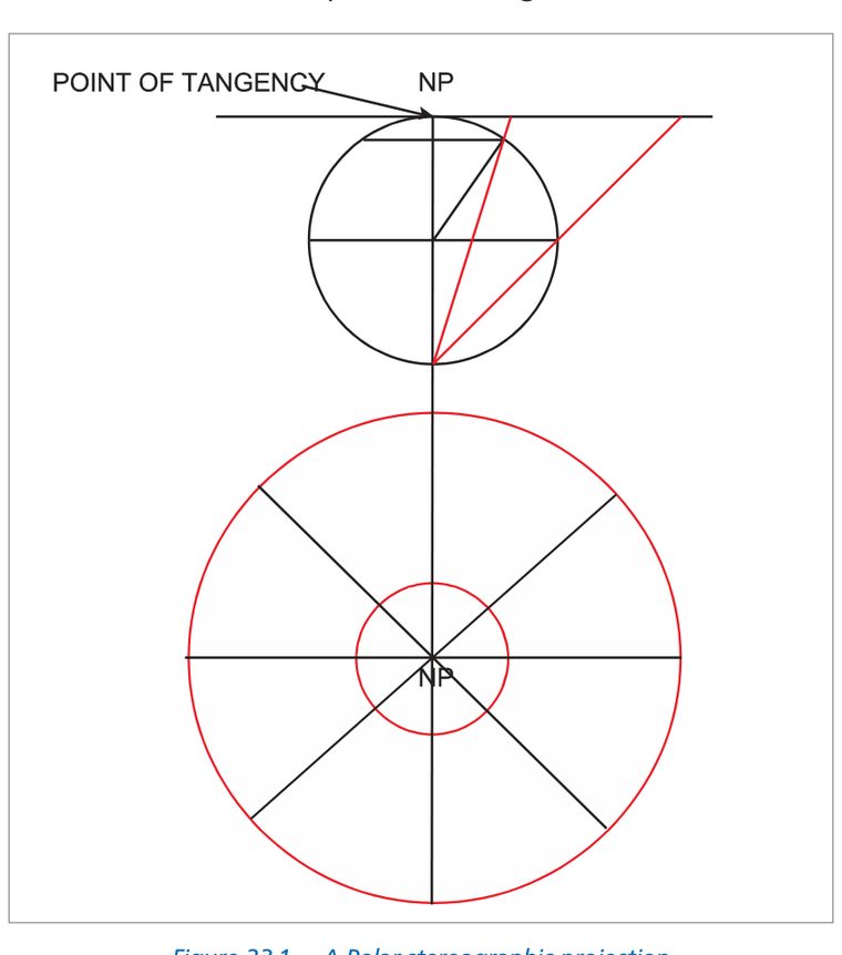
Figure 1 — Polar Stereographic projection construction: flat sheet touches the North Pole; light source at South Pole; the graticule is projected geometrically outward from the pole
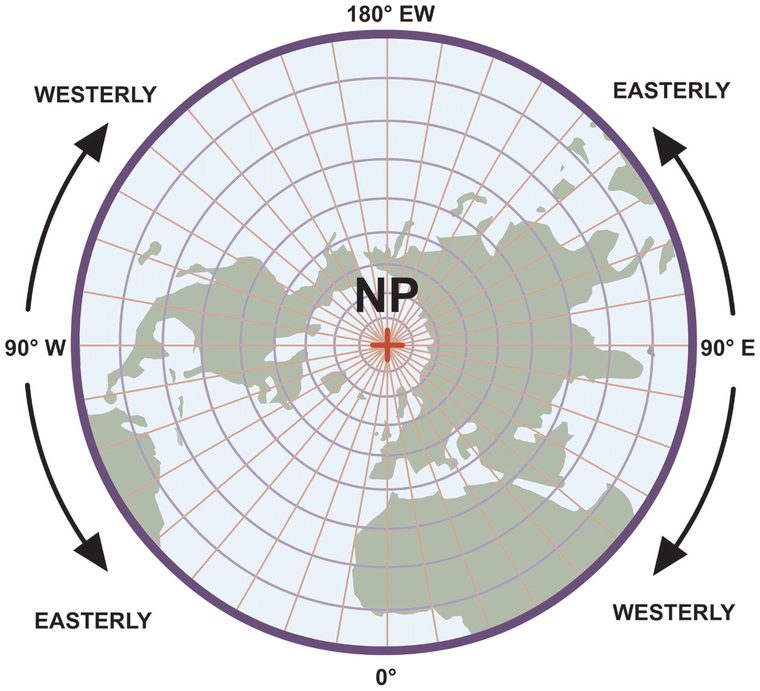
Figure 2 — Polar Stereographic graticule: meridians are straight lines radiating from the pole; parallels are concentric circles; the spacing between parallels increases with distance from the pole
The Co-latitude
The co-latitude is a key concept for polar chart calculations:
Examples:
- Latitude 90°N (the North Pole): co-latitude = 0°
- Latitude 78°N: co-latitude = 12°
- Latitude 70°N: co-latitude = 20°
- Latitude 60°N: co-latitude = 30°
- Latitude 0° (Equator): co-latitude = 90°
The co-latitude is used because polar chart properties (scale expansion, distance from the pole) are measured from the pole rather than the Equator.
Scale Expansion
Scale is correct at the Pole (the point of tangency). Elsewhere it expands with increasing co-latitude (i.e. with decreasing latitude / distance from the pole):
Worked Example — Scale at 78°N
If scale at Pole = 1:1 000 000:
Scale at 78°N = (1/1 000 000) × sec²(6°) = (1/1 000 000) × (1/cos 6°)² = (1/1 000 000) × (1/0.9945)²
= (1/1 000 000) × (1.00554)² ≈ (1/1 000 000) × 1.011 = 1/989 074
→ Scale change from 90°N to 78°N: less than 1%. Chart is within 1% of correct scale.
Scale Zones
The near-constant scale near the pole makes this chart ideal for polar flying:
- 90° to 78°N: Scale within 1% of correct (Pole scale)
- 78° to 70°N: Scale within 3% of correct
- Below 70°N: Scale error exceeds 3%; the chart becomes less suitable
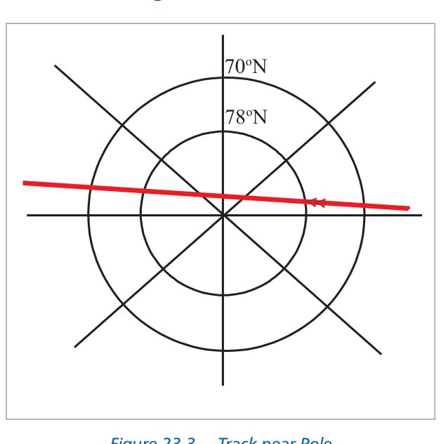
Figure 3 — Scale zones on the Polar Stereographic: the 78°N parallel marks the 1% boundary and the 70°N parallel marks the 3% boundary — this 1% zone covers about 720 NM radius from the pole
The practical significance: the 1% scale zone extends from the Pole to 78°N. The distance from Pole to 78°N = 12° × 60 NM = 720 NM. An aircraft crossing the polar region (entering on one side, exiting the other) travels about 1 400 NM in the 1% zone — approximately 3 hours at typical jet speeds. A chart useful for 3 hours of polar flying with minimal scale error is extremely practical.
Chart Properties
| Property | Detail |
|---|---|
| Projection type | Azimuthal (plane), geometric (perspective), orthomorphic |
| Orthomorphism | Yes — meridians radiate from pole, parallels are concentric circles; expansion is equal in all directions from any point, satisfying both orthomorphism conditions |
| Scale | Correct at Pole. Expands as sec²(½ co-lat). Within 1% from 90°N to 78°N; within 3% from 78°N to 70°N |
| Graticule | Meridians: straight lines from pole. Parallels: concentric circles centred at pole (uneven spacing — wider apart with distance from pole) |
| Shape distortion | Shapes and areas become increasingly distorted away from the pole |
| Practical use | Polar route planning and plotting; ETOPS operations over polar areas; some meteorological charts |
Chart Convergence — n = 1
On the Polar Stereographic chart, the meridians converge at the pole at exactly the same rate as they do on the Earth's surface. This gives the chart a convergence factor n = 1:
On the real Earth, convergency = ch.long × sin(latitude). At the Pole, sin(90°) = 1, so Earth convergency = ch.long. Chart convergence (always = ch.long) equals Earth convergency only at the Pole. Elsewhere, chart convergence > Earth convergency (since sin(lat) < 1 at any latitude other than the Pole).
n = 1: The Key Number for Polar Stereo Problems
For any two meridians on a Polar Stereographic chart, the angle between them on the chart = their difference in longitude. This is the starting point for all straight-line track problems on this projection.
Rhumb Lines and Great Circles
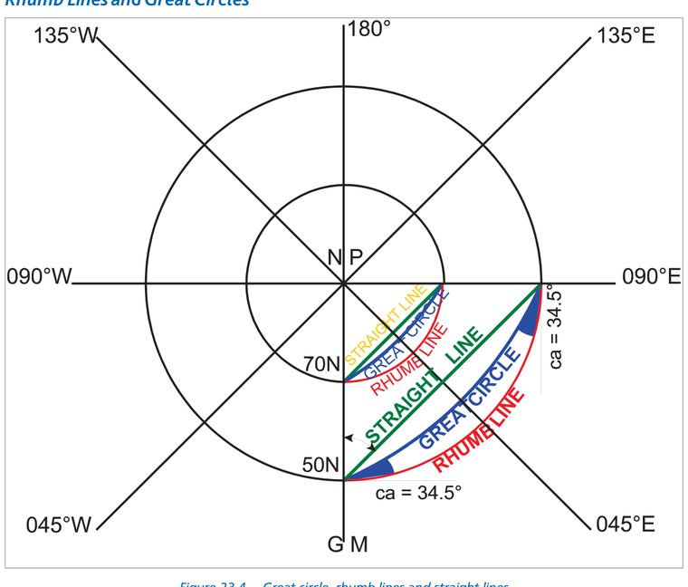
Figure 4 — Great circles, rhumb lines and straight lines on a Polar Stereographic chart between two meridians (000°E and 090°E) at 50°N and 70°N — the straight line on the chart sits between the RL and GC in terms of curvature
Rhumb Lines
Rhumb lines are curves concave to the Pole (same as on the Lambert chart, but here the "Parallel of Origin" is the pole itself). The curvature is considerable.
Great Circles
Great circles are also curves concave to the Pole, but with less curvature than Rhumb Lines in the same hemisphere.
Straight Lines vs Great Circles at Different Latitudes
The difference between a straight line on the chart and the corresponding Great Circle can be calculated:
- At 50°N, 90° ch.long: Angle between straight line and RL = ½ × chart convergence = ½ × 90° = 45°. Conversion angle = ½ × 90 × sin(50°) = 34.5°.
Difference = 45° − 34.5° = 10.5°. Too large to treat as equal. - At 70°N, 90° ch.long: ½ CC = 45°. Conversion angle = ½ × 90 × sin(70°) = 42.3°.
Difference = 45° − 42.3° = 2.7°. Acceptably small.
Rule of Thumb
At latitudes above 70°N (or 70°S), a straight line on a Polar Stereographic chart may be taken as a Great Circle. Below 70°N, the approximation breaks down.
Straight-line Track Problems
These are the most common exam questions on this chapter. Two methods work:
- Triangle geometry: Draw the triangle formed by the Pole, point A, and point B. Use the fact that the angle at the Pole = ch.long (since n = 1). Solve the triangle (isosceles if A and B are at the same latitude).
- Rhumb Line method: Find the RL track (easy — same latitude means 090° or 270°). Then subtract half chart convergence to find the initial straight-line track.
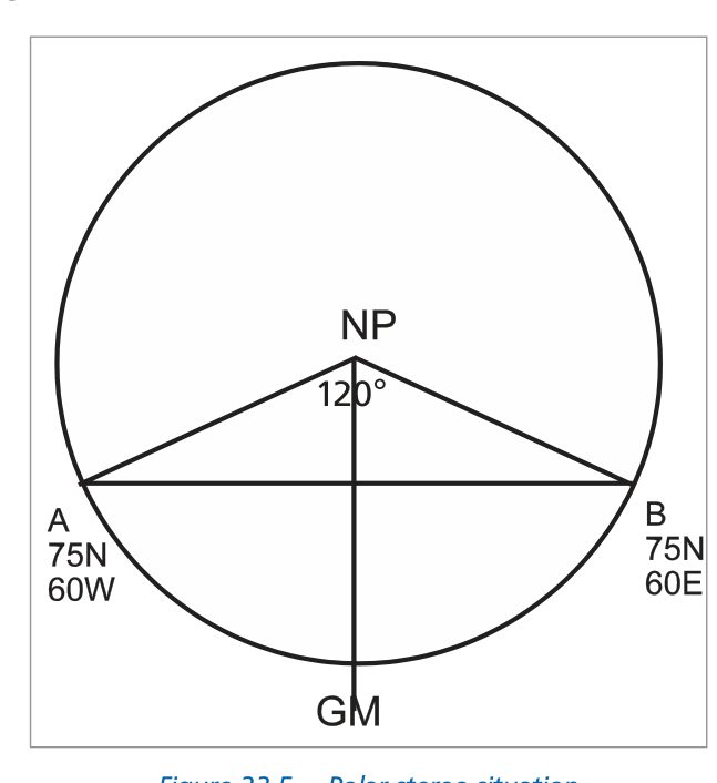
Figure 5 — Example 1 diagram — isosceles triangle A(75N 60W)–Pole–B(75N 60E); apex angle = 120° (ch.long); base angles each = 30°
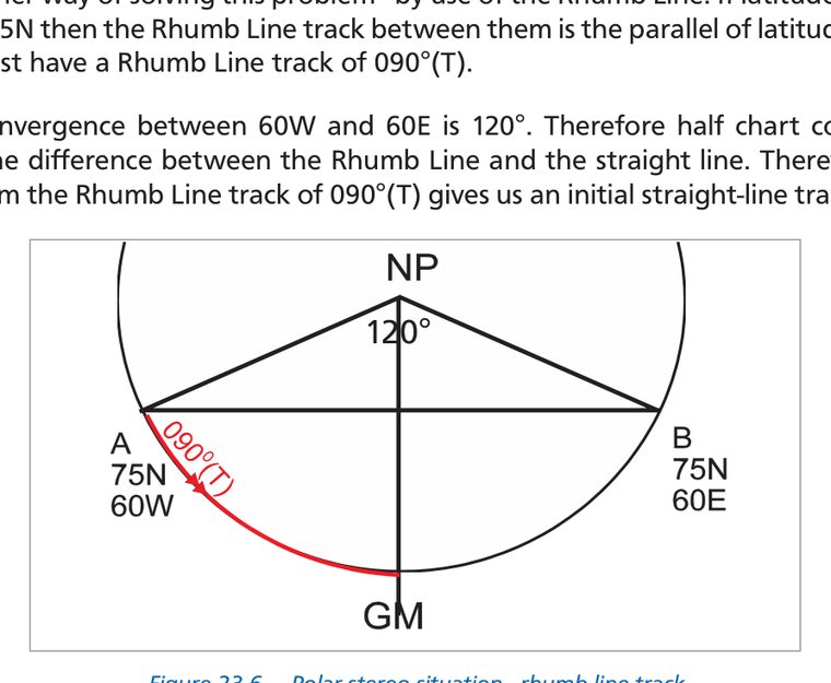
Figure 6 — Example 1 using the RL method — RL track = 090°(T); half chart convergence = 60°; straight-line track at A = 090° − 60° = 030°(T)
Example 1: Initial straight-line track from A (75N 60W) to B (75N 60E)
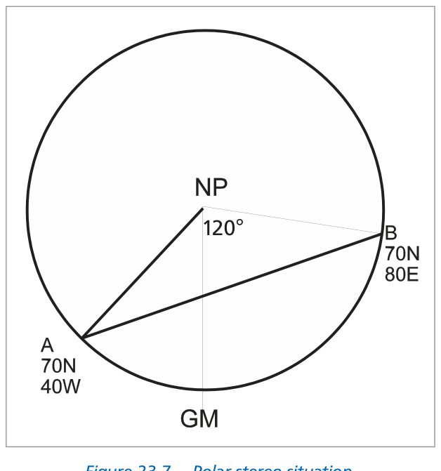
Figure 7 — Example 2 — vertex longitude: the highest latitude on a straight line between two points occurs at the shortest distance from the Pole, where the perpendicular from the Pole meets the line
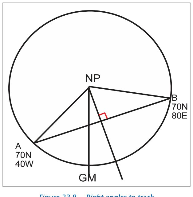
Figure 8 — Example 2 — perpendicular from Pole to track meets at mid-meridian (020°E = mid-point of 40°W and 80°E)
Example 2: Highest latitude on straight-line from A (70N 40W) to B (70N 80E)
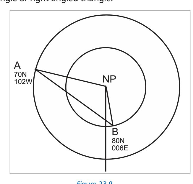
Figure 9 — Example 3 setup — A (70N 102W) and B (80N 006E) at different latitudes; highest latitude along the line is at 035°W
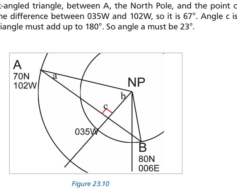
Figure 10 — Example 3 solution — the perpendicular from the Pole to the highest-latitude point creates a right-angled triangle; angle b = 102°W − 035°W = 67°; angle a = 180° − 90° − 67° = 23°
Example 3: Initial track from A (70N 102W) to B (80N 006E) — highest latitude at 035°W
Summary — Properties of a Polar Stereographic Chart
| Projection type | Azimuthal (flat sheet), geometric/perspective, orthomorphic |
| Scale | Correct at Pole. Elsewhere expands as sec²(½ co-lat). Within 1%: 90°→78°. Within 3%: 78°→70°. |
| Graticule | Meridians: straight lines from Pole. Parallels: concentric circles (uneven — increasingly spaced). |
| Orthomorphic | Yes — equal scale expansion in all directions at any point. |
| Chart Convergence | = ch.long. Constant everywhere. Correct only at the Pole. n = 1. |
| Rhumb Lines | Curves concave to the Pole (except meridians). |
| Great Circles | Curves concave to the Pole, but with less curvature than RLs. Treated as straight lines above 70°. |
| Straight-line track | Initial track at A = 000°(T to Pole) ± angle from isosceles/right-angle triangle. Or: RL ± half CC. |
Reinforce Chapter 14: The Polar Stereographic Chart
Test your knowledge and practice actual exam questions for Air Navigation.